If you don't use it you lose it.

It's been a while since I needed to write some data processing scripts. And boy am I rusty! Here is the script I wrote to average out 40 samples per data point on a wafer map, and outputting the results in an Excel spreadsheet. 

#!perl
# processResistivityMap.pl
# Take 40-pt Kelvin Resistivity Data and generate single resistivity per location on wafer.
# Works with one data file at a time representing the wafer map.
# Jovan Trujillo
# Advanced Electronics and Photonics Core Facility
# Arizona State University
# 3/20/2024
# Changelog
# v1.0 - Use last point in 40-pt data file for resistivity map output.
# v1.1 - Added k correction factor to analysis() subroutine.
# v1.2 - Parse X,Y,Z and Temperature from file.

use Modern::Perl;
use File::Find;
use Switch;
use Excel::Writer::XLSX;
our $Excelbook;
our $Excelsheet;
our $row;
our $col;

sub main {
    if ($#ARGV != 1) {
        print "Usage: perl processResistivityMap.pl path-to-data-file output-file-name\n";
    } else {
       
        # ControlPanel will provide interface for Excel Macros embedded into the data collected into this spreadsheet. Will be useful for generating the plots I want, unless PDL can do it more efficiently for me.
        # Need to write some chart making macros in Excel and export the VBA as a binary. The Excel::Writer::XLSX module has a program to help me do that.
        # From the command line.
        my $file = shift @ARGV;
        my $outputName = shift @ARGV;
        $Excelbook = Excel::Writer::XLSX->new($outputName);
                die "Problems creating new Excel file: $!" unless defined $Excelbook;
        $Excelsheet = $Excelbook->add_worksheet('Summary');
        $row = 0;
        $col = 0;
       
        $Excelsheet->write($row,0,"X (um)");
    
        $Excelsheet->write($row,1,"Y (um)");
    
        $Excelsheet->write($row,2,"Z (um)");
    
        $Excelsheet->write($row,3,"T (deg C.");
    
        $Excelsheet->write($row,4,"R (Ohms/sq)");
        $row = $row + 1;
       
        print "\n\nSearching for resistivity data in: " . $file . "\n\n";
        &process_file($file);
        $Excelbook->close();
    }
}

sub process_file {
    #print "filepath: " . $File::Find::name . "\n";
    my $filepath = shift @_;
    my $sampleNum;
    my $wafer;
    my $lotName;
    #my $Excelbook = shift @_;
    
    #my $filename;
    #print "filename: $filename\n";
    if ( -f $filepath) {
        # print " This is a file : $filename \n";
        &analysis($filepath);
    } else {
        # Keep looking for valid data files.
        say "Not a valid file path\n";
    }
}

sub analysis() {
    my $filepath = shift @_;
    #my $filename = shift @_;
    #my $sampleNum = shift @_;
    #my $wafer = shift @_;
    #my $lotName = shift @_;
    #my $Excelbook = shift @_;
    my $DI;
    my $DV;
    my $AV;
    my $CV;
    
    my $Vdiff;
    my $Temperature;
    my $Resistivity=0.0;
    my $count=0;
    my $sum=0;
    my $k = 1;
    my $x;
    my $y;
    my $z;
    
    open DATA, "<$filepath" or die "Error opening file $filepath: $!\n";
    #$header = <DATA>;
    
    while (my $line = <DATA>) {
        # We skip the first 10 points of resistivity data and average out the rest. Or try just the last point. Want to see which
        # analysis will give us the best uniformity.
        if ( $line =~  /\(([\d.]+),([\d.]+),([\d.]+)\)\s*([\d.]+)C\s*/ ) {
            say "\nFound coordinates\n";
            if ($count > 0) {
                print "Average Resistance = " . $sum/$count . "\n";
                $Excelsheet->write($row,4,$sum/$count);
                $sum = 0;
                $count = 0;
                $row = $row + 1;
            }
            $x = $1;
            $y = $2;
            $z = $3;
            $Temperature = $4;
            say "x = $x";
            say "y = $y";
            say "z = $z";
            say "Temperature = $Temperature";
            $Excelsheet->write($row,0,$x);
            $Excelsheet->write($row,1,$y);
            $Excelsheet->write($row,2,$z);
            $Excelsheet->write($row,3,$Temperature);
           
           
        } else {
            if ($line =~ /C|Resistivity|Inf|^\s*$/) {
                #say "Found header line. Skipping it.";
            } else {
                #say "Reading data from: $line";
                ($DI,$DV,$CV,$AV,$Resistivity) = split(/\t\s*/,$line,5);
                # say "DI = $DI";
                # say "DV = $DV";
                # say "CV = $CV";
                # say "AV = $AV";
                #say "Resistivity = $Resistivity";
                $sum = $sum + $Resistivity;
                $count = $count + 1;
               
            }
        }
    }
    
    if ($count > 0) {
        print "Average Resistance = " . $sum/$count . "\n";
        $Excelsheet->write($row,4,$sum/$count);
        $sum = 0;
        $count = 0;
        $row = $row + 1;
    }

    # Save data to Excel Workbook
    #Columns are:
    # 0 - x
    # 1 - y
    # 2 - z
    # 3 - temperature
    # 4 - resistivity
    
    say "All done!";
    close(DATA);
}


    
    

&main();
1;

I had trouble remembering my regex syntax, and the data input file had some sneaky spaces in places that took me a while to see. But in the end I got it to work, after an afternoon and a morning working on it.

 

QBasic in action! Why I chose QBasic at work to develop drafting solutions.

It's been a very long time since I used QBasic for exploring graphics. But this week I need to learn how to do just that for a drafting assignment I had at work. I need to modify a semiconductor circuit layout for a new connector, and that required re-routing over 320 bus lines in the drawing. I wasn't going to do that manually, so I needed to learn the scripting language for this software. So that's when I turned to QBasic, both modern and old, to develop my very own "fanout" algorithm.

That drafting software is called DW-2000 and it's completely new to me. I was just learning how it's scripting language, GPE, can be used to draw when I was given this assignment. I didn't think I was comfortable enough with the language to work out the fanout algorithm in it. I usually work out ideas in Perl or LabView, or even Excel if I'm just looking at data. But for graphical stuff? The first language that came to my mind was also the very first one I learned about as a little kid, QBasic. 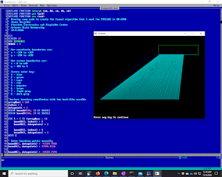So I fired up QB64, the working man's modern QBasic, and got to work drawing polygons and lines to test out how I was going to write this code in GPE. That's an early example of what I was doing in the picture. Eventually the fanout needed to be more complicated than a simple A to B connection, and I did those final tweaks in GPE after learning how to draw path-lines in it from some example code that DW-2000 provides. GPE is a very interesting language as well. It's an array language that operates in a way that totally reminds me of the J programming language. I'm really glad I've played around with J for years before coming across GPE. It really made it much easier for me to wrap my head around the syntax of it. So without much ado I give you some QBasic code, which works on modern QB64 and old school QBasic 4.5.

DECLARE FUNCTION interp# (a#, B#, c#, d#, x#)
DECLARE FUNCTION ys% (yc#)
DECLARE FUNCTION xs% (xc#)
' Develop some code to create the fanout algorithm that I want for FDC13SS in DW-2000
' Jovan Trujillo
' Flexible Electronics and DisplaY#s Center
' Arizona State University
' 12/1/2020

CLS
SCREEN 12
REM $DYNAMIC
DEBUG = 0

' Our coordinate boundaries are:
' x = -320 to +320
' y = -240 to +240
'
' Our screen boundaries are:
' x = 0 to 640
' y = 480 to 0
'
' Screen color key:
' 1 - blue
' 2 - green
' 3 - cyan
' 4 - red
' 5 - magenta
' 6 - brown
' 7 - light gray
' 8 - dark gray

'Declare boundary coordinates with two hash-like arraY#s
arrayMax% = 500
index% = 0
datapoint% = 1
REDIM boundX(500, 2) AS DOUBLE
REDIM boundY(500, 2) AS DOUBLE

FOR I = 0 TO (arrayMax% - 1)
    boundX(I, index%) = I
    boundX(I, datapoint%) = 0

    boundY(I, index%) = I
    boundY(I, datapoint%) = 0
NEXT I

' Enter boundary points manually
boundX(0, datapoint%) = -43104.998#
boundY(0, datapoint%) = 23900.031#

boundX(1, datapoint%) = -43104.737#
boundY(1, datapoint%) = 25096.649#

boundX(2, datapoint%) = -1980.657#
boundY(2, datapoint%) = 36489.974#

boundX(3, datapoint%) = 34770.5#
boundY(3, datapoint%) = 36489.974#

' Let's rescale these points to our screen resolution
boundPointCount% = 4

minYLayout# = boundY(0, datapoint%)
maxYLayout# = boundY(0, datapoint%)
minXLayout# = boundX(0, datapoint%)
maxXLayout# = boundX(0, datapoint%)

minXScreen# = 0!
maxXScreen# = 639!
minYScreen# = 479!
maxYScreen# = 0!

minXCart# = -320!
maxXCart# = 320!
minYCart# = -240!
maxYCart# = 240!

FOR I = 0 TO (boundPointCount% - 1)
    IF boundX(I, datapoint%) < minXLayout# THEN
        minXLayout# = boundX(I, datapoint%)
    END IF

    IF boundX(I, datapoint%) > maxXLayout# THEN
        maxXLayout# = boundX(I, datapoint%)
    END IF

    IF boundY(I, datapoint%) < minYLayout# THEN
        minYLayout# = boundY(I, datapoint%)
    END IF

    IF boundY(I, datapoint%) > maxYLayout# THEN
        maxYLayout# = boundY(I, datapoint%)
    END IF
NEXT I

minXLayout# = minXLayout# - 5000
minYLayout# = minYLayout# - 5000
maxXLayout# = maxXLayout# + 5000
maxYLayout# = maxYLayout# + 5000

IF DEBUG = 1 THEN
    PRINT "minXLayout: ", minXLayout#
    PRINT "minYLayout: ", minYLayout#
    PRINT "maxXLayout: ", maxXLayout#
    PRINT "maxYLayout: ", maxYLayout#
END IF


' Use interp to do the scaling, let's draw the boundary!
aX# = minXLayout#
bX# = minXCart#
cX# = maxXLayout#
dX# = maxXCart#

aY# = minYLayout#
bY# = minYCart#
cY# = maxYLayout#
dY# = maxYCart#

sX1 = 0#
sY1 = 0#
sX2 = 0#
sY2 = 0#

FOR I = 0 TO (boundPointCount% - 2)
    sX1# = interp#(aX#, bX#, cX#, dX#, boundX(I, datapoint%))
    sY1# = interp#(aY#, bY#, cY#, dY#, boundY(I, datapoint%))

    sX2# = interp#(aX#, bX#, cX#, dX#, boundX(I + 1, datapoint%))
    sY2# = interp#(aY#, bY#, cY#, dY#, boundY(I + 1, datapoint%))

    IF DEBUG = 1 THEN
        PRINT "I:"; I; " (LX1, LY1) = "; boundX(I, datapoint%); ","; boundY(I, datapoint%)
        PRINT "I: "; I; " (sX1, sY1) = "; xs%(sX1#); ","; ys%(sY1#)
        PRINT "I: "; I + 1; " (LX2, LY2) = "; boundX(I + 1, datapoint%); ","; boundY(I + 1, datapoint%)
        PRINT "I: "; I + 1; " (sX2, sY2) = "; xs%(sX2#); ","; ys%(sY2#)
        PRINT ""
    END IF

    LINE (xs%(sX1#), ys%(sY1#))-(xs%(sX2#), ys%(sY2#)), 1
NEXT I

IF DEBUG = 1 THEN
    ' Test what's going on with interp
    I = 0
    sX1# = interp#(aX#, bX#, cX#, dX#, boundX(I, datapoint%))
    sY1# = interp#(aY#, bY#, cY#, dY#, boundY(I, datapoint%))
    PRINT "(I, LX1, LY1) = "; I; boundX(I, datapoint%); boundY(I, datapoint%)
    PRINT "(I, sX1, sY1) = "; I; sX1#; sY1#
END IF

' Time to draw the tab locations
sX1# = interp#(aX#, bX#, cX#, dX#, 3160.499#)
sY1# = interp#(aY#, bY#, cY#, dY#, 36407.03#)
sX2# = interp#(aX#, bX#, cX#, dX#, 34793.5#)
sY2# = interp#(aY#, bY#, cY#, dY#, 38981.031#)

IF DEBUG = 1 THEN
    PRINT "(LX1#, LY1#, LX2#, LY2#): "; 3160.499#; 36407.03#; 34793.5#; 38981.031#
    PRINT "(sX1#, sY1#, sX2#, sY2#): "; sX1#; sY1#; sX2#; sY2#
    PRINT "(sX1%, sY1%, sX2%, sY2%): "; xs%(sX1#); ys%(sY1#); xs%(sX2#); ys%(sY2#)
END IF

' Draw source tab outline here.
LINE (xs%(sX1#), ys%(sY1#))-(xs%(sX2#), ys%(sY2#)), 2, B

' Draw array tab line here.
sX1# = interp#(aX#, bX#, cX#, dX#, -42993.999#)
sY1# = interp#(aY#, bY#, cY#, dY#, 24190#)
sX2# = interp#(aX#, bX#, cX#, dX#, 39946#)
sY2# = sY1#

LINE (xs%(sX1#), ys%(sY1#))-(xs%(sX2#), ys%(sY2#)), 2


' Now the real work begins! Time to try to draw a fanout!
' Array pitch is 260 um
' Source Tab pitch is 80 um
' Let's say there are 240 lines.
lineCount% = 240
arrayPitch% = 260
sourcePitch% = 80

arrayX1# = -42993.999#
arrayY1# = 24190#
tabX1# = 3970.5#
tabY1# = 36407.031#

FOR I = 1 TO lineCount%
    ' Draw lines from array to source tab
    X1% = xs%(interp#(aX#, bX#, cX#, dX#, arrayX1#))
    Y1% = ys%(interp#(aY#, bY#, cY#, dY#, arrayY1#))
    X2% = xs%(interp#(aX#, bX#, cX#, dX#, tabX1#))
    Y2% = ys%(interp#(aY#, bY#, cY#, dY#, tabY1#))
    LINE (X1%, Y1%)-(X2%, Y2%), 3
    arrayX1# = arrayX1# + arrayPitch%
    tabX1# = tabX1# + sourcePitch%
NEXT I


END

FUNCTION interp# (a#, B#, c#, d#, x#)
    ' Interpolate and return y given x and endpoints of a line
    IF (a# - c#) <> 0 THEN
        slope# = (B# - d#) / (a# - c#)
        intercept# = d# - ((B# - d#) / (a# - c#)) * c#
        interp# = slope# * x# + intercept#
    ELSE
        PRINT "interp cannot divide by zero!"
        interp# = 0#
    END IF

END FUNCTION

FUNCTION xs% (xc#)
    ' Remember that for SCREEN 12 X limites are -320 to 320
    ' Convert Cartesian coordinate system to screen coordinates
    'xs = xc + 320

    IF (xc# > 320) THEN
        xs% = 320
    ELSEIF (xc# < -320) THEN
        xs% = -320
    ELSE
        xs% = INT(xc# + 320)
    END IF
END FUNCTION

FUNCTION ys% (yc#)
    ' Remember that for SCREEN 12 Y limits are -240 to 240
    ' Convert Cartesion coordinate system to screen coordinates
    'ys = 240 - yc

    IF (yc# > 240) THEN
        ys% = 240
    ELSEIF (yc# < -240) THEN
        ys% = -240
    ELSE
        ys% = INT(240 - yc#)
    END IF

END FUNCTION
     
      

And here is the final production code for drafting out the bus lines in GPE.

      \\ fanout.gpe
\\ Hardcoded fanout macro to help us finish FDC13SS design layout
\\ Jovan Trujillo
\\ FEDC - Arizona State University 
\\ 12/3/2020

menu
	"fanout2_parta"
	"fanout2_partb"
endmenu

dyadic function y := endpoints INTERP x
	local slope; intercept; a; b; c; d
	a := endpoints[1]
	b := endpoints[2]
	c := endpoints[3]
	d := endpoints[4]
	slope := (b -d)/(a-c)
	intercept := d - slope * c
	y := slope * x + intercept
endsub

niladic procedure fanout2_parta
	local lineCount; arrayPitch1; tabPitch1; arrayX1; arrayY1; tabX1; tabY1; startPoint1; endPoint1; i; endpoints
	local arrayPitch2; tabPitch2; arrayX2; tabX2; arrayY2; tabY2; startPoint2; endPoint2
	
\\ We do the last 62 lines in fanout_partb, and then connect these lines to the actual tab using fanout_partc and fanout_partd
	lineCount := 258 
	arrayPitch1 := 260.0
	tabPitch1 := 80.0

	endpoints := (2618.325;35407.058;23308.41;28964.53)
	
	arrayX1 := -42994.00
	\\arrayY1 := 24190.00-8.0
	arrayY1 := 24182.00
	tabX1 := 3258.325
	tabY1 := endpoints INTERP tabX1

	arrayPitch2 := 80
	tabPitch2 := 80

	arrayX2 := 3258.325
	arrayY2 := endpoints INTERP arrayX2
	tabX2 := 3258.325
	tabY2 := 36407.058

	
	path       ! datatype 6
	layer 14   ! width 20
	pathtype 0 ! straight
	vlayer 14   ! solid

	startPoint1 := arrayX1, arrayY1
	endPoint1 := tabX1, tabY1
	startPoint2 := arrayX2, arrayY2
	endPoint2 := tabX2, tabY2


	for i range (iota(1,lineCount)) do
		ce startPoint1
		ce endPoint1
		ce startPoint2
		ce endPoint2
		put
		arrayX1 := arrayX1 + arrayPitch1
		tabX1 := tabX1 + tabPitch1
		startPoint1 := arrayX1, arrayY1
		tabY1 := endpoints INTERP tabX1
		endPoint1 := tabX1, tabY1
		tabX2 := tabX2 + tabPitch2
		arrayX2 := arrayX2 + arrayPitch2
		arrayY2 := endpoints INTERP arrayX2
		startPoint2 := arrayX2, arrayY2
		endPoint2 := tabX2, tabY2

	enddo
	
	view

endsub	

niladic procedure fanout2_partb
local lineCount; arrayPitch1; tabPitch1; arrayX1; arrayY1; tabX1; tabY1; startPoint1; endPoint1; i; endpoints
local arrayPitch2; tabPitch2; arrayX2; tabX2; arrayY2; tabY2; startPoint2; endPoint2
	
	lineCount := 62
	arrayPitch1 := 260
	tabPitch1 := 80.0
	
	endpoints := (23258.296; 29005.016; 23308.41; 29033.135)

	arrayX1 := 24086.00
	\\arrayY1 := 24190.00 - 8.0
	arrayY1 := 24182.00
	tabX1 := 23898.296
	tabY1 := endpoints INTERP tabX1

	arrayPitch2 := 80
	tabPitch2 := 80

	arrayX2 := 23898.296
	arrayY2 := endpoints INTERP arrayX2
	tabX2 := 23898.325
	tabY2 := 36407.058

	startPoint2 := arrayX2, arrayY2
	endPoint2 := tabX2, tabY2


	
	path       ! datatype 6
	layer 14   ! width 20
	pathtype 0 ! straight
	vlayer 14   ! solid

	startPoint1 := arrayX1, arrayY1
	endPoint1 := tabX1, tabY1

	for i range (iota(1,lineCount)) do
		ce startPoint1
		ce endPoint1
		ce startPoint2
		ce endPoint2
		put
		arrayX1 := arrayX1 + arrayPitch1
		tabX1 := tabX1 + tabPitch1
		startPoint1 := arrayX1, arrayY1
		tabY1 := endpoints INTERP tabX1
		endPoint1 := tabX1, tabY1
		tabX2 := tabX2 + tabPitch2
		arrayX2 := arrayX2 + arrayPitch2
		arrayY2 := endpoints INTERP arrayX2
		startPoint2 := arrayX2, arrayY2
		endPoint2 := tabX2, tabY2
	enddo
	view
endsub	

		
      

Fun stuff. In the future I want to add boundary checking code and some adaptive approach to drawing all those paths so I don't have to think about the geometry. Just give it A and B and the pitch and number of lines and let the code draw the pathways. I'll be using QBasic to help me work all that out as well!

My only use of PureBasic

It was 2015 and I was taking a course on Discrete Event Simulation for my master's degree in computer modeling and simulation. We had a group project and needed to simulate the process flow of an imaginary factory. I though I would implement some of the calculations in PureBASIC  to help me get a taste of the language. It was not too bad. I quickly figured out how to make the procedures, array manipulation, and loops I needed. The final script ended up very useful for the project and I shared it with the rest of the class. I think it's fairly readable even for people who don't know PureBASIC. Here is the little script I wrote long ago.

 Procedure.f sum(Array dataInput(1))
  total.f = 0.0
  For i=0 To ArraySize(dataInput())
    total = total + dataInput(i)
  Next
  ProcedureReturn total
EndProcedure

Procedure.f min(Array dataInput(1))
  min.f = dataInput(0)
  For i=0 To ArraySize(dataInput())
    If dataInput(i) < min
      min = dataInput(i)
    EndIf
  Next
  ProcedureReturn min
EndProcedure

Procedure Main()
  ; myDEBUG = 1 to see more console output
  myDEBUG.l = 0
  ; User interface setup
  OpenConsole()
  EnableGraphicalConsole(1)
  ConsoleLocate(0,0)
  PrintN("makespan calculator started...")
 
  ; Load tool timing data from csv file
  FileName$ = OpenFileRequester("Choose a CSV File", "", "*.csv|*.csv", 0)
 
  If OpenFile(0, FileName$)
    While Not Eof(0)
      line$ = ReadString(0)
      
    Wend
    CloseFile(0)
  EndIf
 
  ;; Calculate makespan for flow shop
  Dim dataTable.f(3,3)
 
  dataTable(0,0) = 2.0
  dataTable(0,1) = 3.5
  dataTable(0,2) = 1.5
  dataTable(0,3) = 2.0
  dataTable(1,0) = 4.5
  dataTable(1,1) = 3.0
  dataTable(1,2) = 2.5
  dataTable(1,3) = 1.0
  dataTable(2,0) = 1.5
  dataTable(2,1) = 1.5
  dataTable(2,2) = 5.0
  dataTable(2,3) = 0.5
  dataTable(3,0) = 4.0
  dataTable(3,1) = 1.0
  dataTable(3,2) = 2.5
  dataTable(3,3) = 0.5
 
  ;; Construct a Gantt chart to show how the makespan is calculated.
  ;; For Example 4.3 from the textbook the desired job sequence is {2,4,1,3}
  NewList jobSeq.l()
  AddElement(jobSeq())
  jobSeq() = 2
  AddElement(jobSeq())
  jobSeq() = 4
  AddElement(jobSeq())
  jobSeq() = 1
  AddElement(jobSeq())
  jobSeq() = 3
 
  PrintN("jobSeq Contents:")
  ForEach jobSeq()
    Print(Str(jobSeq()) + " ")
  Next
  PrintN("")
 
  ResetList(jobSeq())
 
  ;; Now we calculate the makespan using the jobSeq and data from dataTable
  t.f = 0.0
  dt.f = 0.1
  jobsDone.l = 0
  Dim toolTimes.f(3)
  Dim jobAtTool.l(3)
  lastTool.l = 3
 
  ; Initialize arrays
  For i = 0 To ArraySize(toolTimes())
    toolTimes(i) = 0.0
    jobAtTool(i) = 0
  Next
 
  ; Start running the simulation
  While jobsDone < ListSize(jobSeq())
    For i = 0 To ArraySize(toolTimes())
      If i = 0
        ; The first tool will load the next job if idle, and if jobs are available
        ; Make sure the first tool is idle and empty of jobs
        If toolTimes(i) <= 0 And jobAtTool(i) = 0 And NextElement(jobSeq()) <> 0
          jobAtTool(i) = jobSeq()
          toolTimes(i) = dataTable(jobAtTool(i)-1, i)
        EndIf
        
        ; Move time step if there is a job on tool
        If toolTimes(i) > 0
          toolTimes(i) = toolTimes(i) - dt
        Else
          ; do nothing
        EndIf
        
      ElseIf i = ArraySize(toolTimes())
        ; We are in the last tool. Check to see if it has a job and if it is done processing, then we move the job
        ; out and add to jobsDone tally
        If toolTimes(i) <= 0 And jobAtTool(i) <> 0
          jobsDone = jobsDone + 1
          jobAtTool(i) = 0
        EndIf
        
        ; Move previous tools job into current tool if available
        If toolTimes(i-1) <= 0 And jobAtTool(i-1) <> 0 And jobAtTool(i) = 0
          jobAtTool(i) = jobAtTool(i-1)
          jobAtTool(i-1) = 0
          toolTimes(i) = dataTable(jobAtTool(i)-1, i)
        EndIf
      
        ; If there is a job in current tool and there is processing time then move time step forward.
        If toolTimes(i) > 0
          toolTimes(i) = toolTimes(i) - dt
        Else
          ; do nothing
        EndIf
        
      Else
        ; We are after the first tool but before the last
        ; Check if tool is empty but with a job. Then it is done with job.
        ; Check if next tool is empty, if so then move job to next tool.
        ; Check if previous tool is empty. If so then increment time and move on.
        ; Check if previous tool is empty but with a job, then if current tool is empty move job.
        
        ; Move job to next tool if next tool is empty and current tool is done processing
        If jobAtTool(i) <> 0 And jobAtTool(i+1) = 0 And toolTimes(i) <= 0
          jobAtTool(i+1) = jobAtTool(i)
          toolTimes(i+1) = dataTable(jobAtTool(i+1)-1, i)
          jobAtTool(i) = 0
        EndIf
        
        ; Move previous tool's job into current tool if available
        If toolTimes(i-1) <= 0 And jobAtTool(i-1) <> 0 And jobAtTool(i) = 0
          jobAtTool(i) = jobAtTool(i-1)
          toolTimes(i) = dataTable(jobAtTool(i)-1, i)
          jobAtTool(i-1) = 0
        EndIf
        
        ; Increment t and decrement tool's processing time if busy with a job.
        If toolTimes(i) > 0
          toolTimes(i) = toolTimes(i) - dt
        Else
          ; Do nothing
        EndIf
      EndIf
    Next
    
    t = t + dt
    If myDEBUG = 1
      PrintN("t: " + t)
      PrintN("Job Status:")
      For i = 0 To ArraySize(jobAtTool())
        Print(Str(jobAtTool(i)) + " ")
      Next
      PrintN("")
      
      PrintN("jobsDone: " + Str(jobsDone) + " out of " + Str(ListSize(jobSeq())) )
      
      ;PrintN("Tool Times")
      ;For i = 0 To ArraySize(toolTimes())
      ;  Print(Str(toolTimes(i)) + " ")
      ;Next
      ;PrintN("")
      
      ;Delay(500)
    EndIf
    
  Wend
 
  PrintN("makespan: " + t)
  PrintN("Enter key to quit")
  done$ = Input()
  CloseConsole()
  EndProcedure
 
  Main()
 
; IDE Options = PureBasic 5.42 LTS (Windows - x64)
; ExecutableFormat = Console
; CursorPosition = 30
; FirstLine = 15
; Folding = -
; EnableUnicode
; EnableXP

 

Composing with Tandy Model 102 BASIC!

I'm making music people. Here is my debut single available now to download:

https://sweetjehosavan.bandzoogle.com/

I am using my Tandy Model 102 to help me transcribe what I created with the guitar to tabs and sheet music. It's helping me make sure I'm getting all the notes written down and that the timing is correct. Here is the source code so far. I'm not done transcribing the song yet.

 1 'WINDY NIGHT BY JOVAN TRUJILLO
5 G1 = 12538 : G2 = 6269 : G3 = 3134 : G4 = 1567 : G5 = 83
10 N1 = 11836 : N2 = 5918 : N3 = 2959 : N4 = 1479 : N5 = 739
20 BPM = 120
30 BPS = BPM / 60
40 NQ = INT(50/BPS)
50 N8 = NQ/2
60 NH = NQ*2
70 NW = NH * 2
80 A1 = 11172 : A2 = 5586 : A3 = 2793 : A4 = 1396 : A5 = 698
90 H1 = 10544 : H2 = 5272 : H3 = 2636 : H4 = 1318 : H5 = 659
100 B1 = 9952 : B2 = 4976 : B3 = 2488 : B4 = 1244 : B5 = 62
110 C1 = 9394 : C2 = 4697 : C3 = 2348 : C4 = 1174 : C5 = 587
119 ' J IS C#
120 J1 = 8866 : J2 = 4433 : J3 = 2216 : J4 = 1108 : J5 = 554
130 D1 = 8368 : D2 = 4184 : D3 = 2092 : D4 = 1046 : D5 = 523
140 K1 = 7900 : K2 = 3950 : K3 = 1975 : K4 = 987 : K5 = 493
150 E1 = 7456 : E2 = 3728 : E3 = 1864 : E4 = 932 : E5 = 466
160 F1 = 7032 : F2 = 3516 : F3 = 1758 : F4 = 879 : F5 = 439
170 M1 = 6642 : M2 = 3321 : M3 = 1660 : M4 = 830 : M5 = 415
190 FOR X = 1 TO 2
200 SOUND B1, NQ
210 SOUND D2, NQ
220 SOUND B1, N8
230 SOUND A1, NQ
240 SOUND J2, NQ
245 IF X=2 THEN SOUND J2, N8
250 SOUND A1, N8
260 SOUND E1, NQ
270 SOUND G2, NQ
280 SOUND E1, N8
290 SOUND A1, N8
300 SOUND J2, N8
310 SOUND H1, N8
320 SOUND J2, N8
400 NEXT X
405 FOR X = 1 TO 2
410 SOUND B1, NQ
420 SOUND D2, NQ
425 SOUND B1, N8
430 SOUND M3, N8
440 SOUND B2, N8
450 SOUND M2, N8
460 SOUND B1, N8
470 SOUND A1, NQ
480 SOUND J2, NQ
485 SOUND A1, N8
490 SOUND M3, N8
500 SOUND B2, N8
510 SOUND M2, N8
520 SOUND A1, N8
530 SOUND E1, NQ
540 SOUND G2,NQ
545 SOUND G1, N8
550 SOUND M3, N8
560 SOUND B2, N8
570 SOUND M2, N8
580 SOUND A1, NQ
590 SOUND J2, NQ
600 SOUND M3, NH
610 SOUND B1, NQ
620 SOUND D2, N8
630 SOUND B1, N8
640 SOUND B3, N8
650 SOUND B2, N8
660 SOUND M2, N8
670 SOUND B1, N8
680 SOUND A1, NQ
690 SOUND J2, NQ
700 SOUND A1, N8
710 SOUND A3, N8
720 SOUND B2, N8
730 SOUND M2, N8
740 SOUND A1, N8
750 SOUND E1, NQ
760 SOUND G2, NQ
770 SOUND G1, N8
780 SOUND G3, N8
790 SOUND B2, N8
800 SOUND M2, N8
810 SOUND G1, N8
820 SOUND A3, NQ
830 SOUND A3, N8
840 SOUND A3, N8
850 SOUND A3, N8
860 SOUND G3, N8
870 SOUND M3, N8
880 SOUND D2, NQ
890 SOUND B1, NQ
900 SOUND B1, NQ
910 SOUND D2, NQ
915 SOUND B1, N8
920 SOUND B3, N8
930 SOUND M3, N8
935 SOUND B1, N8
940 SOUND A1, NQ
950 SOUND J2, NQ
955 SOUND A1, N8
960 SOUND A3, N8
970 SOUND M3, N8
980 SOUND A1, N8
990 SOUND E1, NQ
1000 SOUND G2, NQ
1010 SOUND G1, N8
1020 SOUND G3, N8
1030 SOUND M3, N8
1035 SOUND A3, NQ
1040 FOR Y = 1 TO 3
1050 SOUND A3, N8
1060 NEXT Y
1070 SOUND G3, N8
1080 SOUND M3, N8
1090 SOUND D2, N8
1100 SOUND B2, N8
1110 SOUND B1, NQ
1120 REM I'm Halfway through this song now! - 5/14/2020

Finding Munchausen Numbers with Perl

Boy has it been forever since I used Perl for something useful. It's been ages since I used Perl for anything actually. And the local Phoenix Perl Mongers group seems to have dissolved as well. That's too bad, because I really did enjoy going to those talks. But if nobody chips in for those talks the group quickly will die out. Eric Tank can only say so many things about the work he does and the things he knows. I wish I knew more about PDL to give a decent talk about it at a new Perl Mongers group meetings. 

But I digress. Today's blog post is a little blurb about Munchausen numbers. It is stated that in the base 10 number system there are only two known Munchausen numbers. I wrote a small Perl script to see if that was true for the numbers ranging form 1 to 500,000. I don't think I ever got to 500,000 before killing the script, but it was fun at least seeing one of the solutions that everyone already agrees upon. I learned some things about number theory. I would like to understand the proof behind the statement of Munchausen numbers. I currently don't understand it. Finding the Wikipedia article about the curious numbers killed my enthusiasm for the Perl script. Instead I had fun running the GAP script a paper provided into my old Debian Panasonic Toughbook So maybe later today I'll post the crappy Perl script I wrote along with the mysterious and amazing GAP code somebody else wrote. LInks and buttons to come in the near future folks! 

Playing with TrueBASIC

I was reading an old book about computer simulation of liquids and wrote this little script that uses the Lennard-Jones potential to calculate the random distribution of atoms in a gas lattice.

OPTION NOLET
! This code illustrates the calculation of the potential energy in a system of
! Lennard-Jones atoms.
! I create a set of atoms in random locations, calculate the Lennard-Jones potential,
! and then move the atoms in a way that would minimize this energy calculation.
N = 20    ! Number of particles
V = 0.0
EPSILON = 164
SIGSQ = .383
STEPX = 0.1
STEPY = STEPX
STEPZ = STEPY
STEP = 1
NOMOVE = 0
InitialPlotString$ = "IP = point(["
FinalPlotString$ = "FP = point(["
filename$ = "output.txt"
OPEN #1: NAME filename$, CREATE NEWOLD
ERASE #1


! Coordinate array for the particles
DIM RX(20)
DIM RY(20)
DIM RZ(20)

! Read coordinate data into arrays
PRINT "Initial atomic positions:"
PRINT "X","Y","Z"
PRINT #1: "Initial atomic positions:"
PRINT #1: "X","Y","Z"
FOR I = 1 TO N
    RX(I) = RND*10
    RY(I) = RND*10
    RZ(I) = RND*10
    PRINT RX(I),RY(I),RZ(I)
    PRINT #1:RX(I),RY(I),RZ(I)
    IF I <> N THEN
        InitialPlotString$ = InitialPlotString$ & "(" & STR$(RX(I)) & "," & STR$(RY(I)) & "," & STR$(RZ(I)) & "),"
    ELSE
        InitialPlotString$ = InitialPlotString$ & "(" & STR$(RX(I)) & "," & STR$(RY(I)) & "," & STR$(RZ(I)) & ")],color=red,size=20,opacity=1)"
    END IF
NEXT I

CALL LennardJones
PRINT "Initial V = "; V
PRINT #1: "Initial V = "; V
OLDV = V
DO WHILE (NOMOVE < 3*N)
    FOR I = 1 TO N
        ! Wiggle atom I in X and see if it reduces the potential.
        RX(I) = RX(I) + STEPX
!        PRINT "STEP ";STEP
        STEP = STEP + 1
        CALL LennardJones

        IF ABS(V) > ABS(OLDV) THEN
            RX(I) = RX(I) - 2*STEPX
!            PRINT "STEP ";STEP
            STEP = STEP + 1
            CALL LennardJones
            IF ABS(V) > ABS(OLDV) THEN
                NOMOVE = NOMOVE + 1
                RX(I) = RX(I) + STEPX
            ELSE
                OLDV = V
            END IF
        ELSE
            OLDV = V
        END IF

        ! Wiggle atom I in Y and see if it reduces the potential.
        RY(I) = RY(I) + STEPY
 !       PRINT "STEP ";STEP
        STEP = STEP + 1
        CALL LennardJones
        IF ABS(V) > ABS(OLDV) THEN
            RY(I) = RY(I) - 2*STEPY
!            PRINT "STEP ";STEP
            STEP = STEP + 1
            CALL LennardJones
            IF ABS(V) > ABS(OLDV) THEN
                NOMOVE = NOMOVE + 1
                RY(I) = RY(I) + STEPY
            ELSE
                OLDV = V
            END IF
        ELSE
            OLDV = V
        END IF

        ! Wiggle atom I in Z and see if it reduces the potential.
        RZ(I) = RZ(I) + STEPZ
        !PRINT "STEP ";STEP
        STEP = STEP + 1
        CALL LennardJones
        IF ABS(V) > ABS(OLDV) THEN
            RZ(I) = RZ(I) - 2*STEPZ
            !PRINT "STEP ";STEP
            STEP = STEP + 1
            CALL LennardJones
            IF ABS(V) > ABS(OLDV) THEN
                NOMOVE = NOMOVE + 1
                RZ(I) = RZ(I) + STEPZ
            ELSE
                OLDV = V
            END IF
        ELSE
            OLDV = V
        END IF
    NEXT I
    PRINT "STEP: ";STEP
LOOP

PRINT "Minimum V: ";OLDV
PRINT "Atomic Coordinates:"
PRINT "X","Y","Z"
PRINT #1: "Minimum V: ";OLDV
PRINT #1: "Atomic Coordinates:"
PRINT #1: "X","Y","Z"
FOR I = 1 TO N
    PRINT RX(I),RY(I),RZ(I)
    PRINT #1: RX(I),RY(I),RZ(I)
    IF I <> N THEN
        FinalPlotString$ = FinalPlotString$ & "(" & STR$(RX(I)) & "," & STR$(RY(I)) & "," & STR$(RZ(I)) & "),"
    ELSE
        FinalPlotString$ = FinalPlotString$ & "(" & STR$(RX(I)) & "," & STR$(RY(I)) & "," & STR$(RZ(I)) & ")], color=blue,size=20,opacity=1)"
    END IF
NEXT I
PRINT #1: "Atomic Positions for Sage plotting:"
PRINT #1: InitialPlotString$
PRINT #1: FinalPlotString$
PRINT #1: "Show(IP+FP)"
PRINT "Done."

SUB LennardJones
! This subroutine calculates the Lennard-Jones potential for the system
LOCAL I
V = 0.0
FOR I = 1 TO N - 1
    RXI = RX(I)
    RYI = RY(I)
    RZI = RZ(I)
    FOR J = I + 1 TO N
        RXIJ = RXI - RX(J)
        RYIJ = RYI - RY(J)
        RZIJ = RZI - RZ(J)

        RIJSQ = RXIJ^2 + RYIJ^2 + RZIJ^2
        SR2 = SIGSQ / RIJSQ
        SR6 = SR2 * SR2 * SR2
        SR12 = SR6^2
        V = V + SR12 - SR6
    NEXT J
NEXT I
V = 4.0 * EPSILON * V
PRINT #1: "STEP "; STEP; ":"
FOR I = 1 TO N
    PRINT #1: RX(I),RY(I),RZ(I)
NEXT I
!PRINT "V = "; V
PRINT #1:"V =";V
END SUB

END

Learning about CBM-BASIC

I've been solving Brilliant math problems with the simplest of BASIC programming languages lately. I do this because it's super convenient for me to write a quick little program to do some equation solving. CBM-BASIC is pretty nice for this because it works with Windows and Linux and my iPhone (by installing Hand-BASIC).

For a nice little example I solved this problem:

 With the help of Mathematica and CBM-BASIC. I used Mathematica to solve for z and plot the resulting equation to help me understand if there were a finite number of solutions. I was being lazy, because I could have figured this out just by plugging a few exploratory numbers in for X,Y, and Z to help me understand the bounds of the problem. Once I understood the bounds of the problem I was able to find all the solutions with CBM-BASIC in a relatively short time period.

Here is the resulting BASIC program:

10 REM Solve Brilliant Problem 2 of May 8, 2017 
20 S = 0
30 E1 = 0
40 MX = 150
50 MY = 50
60 MZ = 40
65 PRINT "FINDING SOLUTIONS..."
70 FOR X = 4 TO MX
80 FOR Y = 1 TO MY
90 FOR Z = 1 TO MZ
100 GOSUB 500
110 IF ABS(E1) < 0.1 THEN S=S+X+Y+Z : PRINT "S = ";S
120 NEXT Z : NEXT Y : NEXT X
130 PRINT "DONE." : END
500 REM EVALUATE FUNCTION E1
510 E1 = X^2*(Y^3+Z^3)-315*(X*Y*Z+7)
520 RETURN

And there you have it. I'll let the reader build CBM-BASIC and find the solution themselves. I'm having a lot of fun using this little Commordore 64 BASIC 2 implementation for my mental exercise. Who said BASIC causes brain damage?

Unicon benchmark results on Raspberry Pi Zero W

This was from a version of Unicon compiled from unicon-code-5082-trunk. A recent development snapshot.


Times reported below reflect averages over three executions.
Expect 2-20 minutes for suite to run to completion.

Word Size  Main Memory  C Compiler  clock    OS         
32 bit     424 MB       gcc 4.9.2   1.0 GHz  UNIX       

CPU                            
1x ARMv6-compatible processor rev 7 (v6l)                  

                                        Elapsed time h:m:s        |Concurrent |
benchmark                           |Sequential|   |Concurrent|   |Performance|
concord concord.dat                   01:0.685            N/A
deal 50000                            01:0.504            N/A
ipxref ipxref.dat                        35.286            N/A
queens 12                             01:13.523            N/A
rsg rsg.dat                           01:3.325            N/A
binary-trees 14                       01:36.725       04:55.517         0.327x
chameneos-redux 65000                      N/A       01:8.534
fannkuch 9                            01:8.319            N/A
fasta 250000                          01:22.580            N/A
k-nucleotide 150-thou.dat             03:19.441            N/A
mandelbrot 750                        08:10.612       13:54.547         0.587x
meteor-contest 600                    03:30.708            N/A
n-body 100000                         03:4.327            N/A
pidigits 7000                         14:37.462            N/A
regex-dna 700-thou.dat                01:52.136       03:33.752         0.524x
reverse-complement 15-mil.dat 
Run-time error 306
File reverse-complement.icn; Line 35
inadequate space in string region
Traceback:
   main(list_1 = [])
   getavgtimes(procedure run_reversecomplement,"15-mil.dat") from line 186 in run-benchmark.icn
   run_reversecomplement(list_5068944 = ["15-mil.dat"]) from line 129 in auxiliary.icn
   mapseq(">ONE Homo sapien...") from line 46 in reverse-complement.icn
   "
Run-time error 302
File reverse-complement.icn; Line 35
memory violation
Traceback:
   main(list_1 = [])
   getavgtimes(procedure run_reversecomplement,"15-mil.dat") from line 186 in run-benchmark.icn
   run_reversecomplement(list_5068944 = ["15-mil.dat"]) from line 129 in auxiliary.icn
   mapseq(">ONE Homo sapien...") from line 46 in reverse-complement.icn

Investigating Bayesian Network Modeling with Perl

I have a capstone project to finish this semester in order to get my Masters of Science in Engineering degree for Modeling and Simulation. It involves modeling a semiconductor fab using a combination of Bayesian network statistics and discrete event simulation. So far I'm in the literature review stage, although I do have a partially working discreet event simulation (DEVS) working from a previous course I took. So I was wondering how I'm going to run the Bayesian network analysis, and if there are any free open source packages already created for me to use. Well, it turns out that there is not much for Bayesian networks. Someone had asked this question on the Perl Monks forum Perl Monks forum but at that time they suggested the application was better suited using fuzzy logic or a naive-Bayes classifier. So per their advice I installed AI::FuzzyInference and AI::Categorizer::Learner::NaiveBayes onto my desktop. I have not had a chance to learn how to use them yet, but when I do I will be sure to document it here.

Check out Notebook Stories for a chance to win Monologue Notebooks!

My first application of the Perl Data Language

I've been installing and testing and playing with PDL for a few years now, but I've never had a need to use it for anything at work. Until now! Recently I needed to update the coordinate file for a set of devices to test. The layout editor showed that the centers of the devices were not rectangular shapes but polygons instead. That made it difficult for the software to give me a central coordinate of the object. What L-Edit does give me though are the vertices of the polygon that makes up that object, and that data was easy enough for me to copy and paste into TextPad. With a few regular expressions and search/replace commands I was able to format the data in a way that Perl could read. I then used PDL to quickly calculate the centroid of the coordinate set, and voila! I had my center coordinate for the device I needed to test. It was my first real use of PDL and I think it saved me a few lines of code. The cool thing was turning it into a PDL function, which could be called by the PDL REPL.

#!/usr/bin/env perl
use Modern::Perl;
use PDL;

sub FDC53_NE_9x9_X4Y0_Centroid() {
    my @V;
    push @V, [53028.301,22242.396];
    push @V, [53028.477,22241.163]; 
    push @V, [53028.532,22240.839];
    push @V, [53028.646,22240.268]; 
    push @V, [53028.958,22239.265];
    push @V, [53029.368,22238.308]; 
    push @V, [53029.672,22237.713];
    push @V, [53029.932,22237.280]; 
    push @V, [53030.687,22236.313];
    push @V, [53031.811,22235.189]; 
    push @V, [53032.783,22234.430];
    push @V, [53033.207,22234.176]; 
    push @V, [53033.814,22233.865];
    push @V, [53034.769,22233.456]; 
    push @V, [53035.763,22233.147];
    push @V, [53036.373,22233.025]; 
    push @V, [53036.628,22232.982];
    push @V, [53037.896,22232.801]; 
    push @V, [53038.608,22232.750];
    push @V, [53127.893,22232.750]; 
    push @V, [53128.603,22232.800];
    push @V, [53129.865,22232.981]; 
    push @V, [53130.134,22233.027];
    push @V, [53130.732,22233.147]; 
    push @V, [53131.735,22233.458];
    push @V, [53132.692,22233.868]; 
    push @V, [53133.287,22234.172];
    push @V, [53133.720,22234.432]; 
    push @V, [53134.687,22235.187];
    push @V, [53135.815,22236.315]; 
    push @V, [53136.566,22237.277];
    push @V, [53136.824,22237.707]; 
    push @V, [53137.134,22238.314];
    push @V, [53137.544,22239.270]; 
    push @V, [53137.852,22240.262];
    push @V, [53137.972,22240.861]; 
    push @V, [53138.020,22241.141];
    push @V, [53138.199,22242.396]; 
    push @V, [53138.250,22243.108];
    push @V, [53138.250,22332.893]; 
    push @V, [53138.200,22333.603];
    push @V, [53138.019,22334.865]; 
    push @V, [53137.973,22335.134];
    push @V, [53137.853,22335.732]; 
    push @V, [53137.542,22336.735];
    push @V, [53137.132,22337.692]; 
    push @V, [53136.828,22338.287];
    push @V, [53136.568,22338.720]; 
    push @V, [53135.813,22339.687];
    push @V, [53134.681,22340.819]; 
    push @V, [53133.727,22341.564];
    push @V, [53133.293,22341.824]; 
    push @V, [53132.686,22342.135];
    push @V, [53131.731,22342.544]; 
    push @V, [53130.737,22342.853];
    push @V, [53130.127,22342.975]; 
    push @V, [53129.872,22343.018];
    push @V, [53128.604,22343.199]; 
    push @V, [53127.892,22343.250];
    push @V, [53038.607,22343.250]; 
    push @V, [53037.897,22343.200];
    push @V, [53036.635,22343.019]; 
    push @V, [53036.366,22342.973];
    push @V, [53035.768,22342.853]; 
    push @V, [53034.765,22342.542];
    push @V, [53033.808,22342.132]; 
    push @V, [53033.213,22341.828];
    push @V, [53032.780,22341.568]; 
    push @V, [53031.813,22340.813];
    push @V, [53030.686,22339.686]; 
    push @V, [53029.933,22338.722];
    push @V, [53029.676,22338.293]; 
    push @V, [53029.365,22337.686];
    push @V, [53028.956,22336.731]; 
    push @V, [53028.647,22335.737];
    push @V, [53028.525,22335.127]; 
    push @V, [53028.482,22334.872];
    push @V, [53028.301,22333.604]; 
    push @V, [53028.250,22332.892];
    push @V, [53028.250,22243.108]; 
   
    my $data = pdl(@V);
    my $mySums = sumover $data->xchg(0,1);
    my @dims = $data->dims;
    return $mySums / $dims[1];
}
       
1;

Converting Excel Macros to Perl

I'm currently working on porting our Excel macros at work to LabView. To get a quick prototype up and running I have been translating the Visual Basic code and the formulas in all of the spreadsheet cell to Perl 6. In the process I get to learn more about Perl 6 and see what all the fuss is about. The Excel macro takes a directory of data files from our transistor testing procedure and extracts certain model parameters for our design engineers. The data is located in tab separated plain text files. They contain voltage and current data for different aspects of the transistor. Each folder contains the data of over a dozen transistors. Here is what I've done so far:

#!/usr/bin/env perl6
use v6;

my $Append = False;
my $Test_Descriptor_Keys_File = "(compute)";
my $Lot_ID = "E1517-002";
my @Wafer_List = "Wafer_11", "Wafer_12";
my @Analysis_Master_Name = "AnalysisMaster_Autoprobe_Prod_20111005";
my $Test_Name_For_Processing = "COW";
my $Path_To_Data_File = "./";
my $Process_Reverse_Sweeps = 1;  my $Print_Graphs = 1;
my $Print_Graphs_To_File = 1;
my $Delete_Summary_Filename_Sheets = 0;
my %Environment = Lot_ID => $Lot_ID, Wafer_List => @Wafer_List, Path_To_Data_File => $Path_To_Data_File,
    Test_Name_For_Processing => $Test_Name_For_Processing, Analysis_Master_Name => $Analysis_Master_Name,
    Test_Descriptor_Keys_File => $Test_Descriptor_Keys_File, Append => $Append, Process_Reverse_Sweeps => $Process_Reverse_Sweeps,
    Print_Graphs => $Print_Graphs, Print_Graphs_To_File => $Print_Graphs_To_File, Delete_Summary_Filenames_Sheets => $Delete_Summary_Filename_Sheets;

sub main() {
    say "Starting...";
    my $myReturn = 1;
    my $myInput = "";
    my $PrintGraphsStatus = "(yes)";
    my $PrintGraphsToFileStatus = "(yes)";
    my $ProcessReverseSweeps = "(yes)";
    my $AppendDataToSummary = "(no)";

    while ($myReturn) {
        say "Choose Function: ";
        say "1. Process TFT Autoprobe Data";
        say "2. Process TFT Princeton Data";
        say "3. Print Graphs? " ~ $PrintGraphsStatus;
        say "4. Print Graphs to File? " ~ $PrintGraphsToFileStatus;
        say "5. Process TFT Data";
        say "6. Delete Summary & Filenames Sheets";
        say "7. Process Reverse Sweeps " ~ $ProcessReverseSweeps;
        say "8. Append Data to Summary " ~ $AppendDataToSummary;
        say "9. Quit";

        $myInput = get();

        given ($myInput) {
            when 1 { $myReturn = &Process_TFT_Autoprobe_Data(%Environment); }
            when 2 { $myReturn = &Process_TFT_Princeton_Data(%Environment); }
            when 3 { $myReturn = &Print_Graphs(%Environment); }
            when 4 { $myReturn = &Print_Graphs_To_File(%Environment); }
            when 5 { $myReturn = &Process_TFT_Data(%Environment); }
            when 6 { $myReturn = &Delete_Summary_Filenames_Sheets(%Environment); }
            when 7 { $myReturn = &Process_Reverse_Sweeps(%Environment); }
            when 8 { $myReturn = &Append_Data_to_Summary(%Environment); }
            when 9 { exit(0); }
            default { $myReturn = 1; }
        }
    }
}

sub Process_TFT_Autoprobe_Data() {
    my %Environment = shift;
    my $Lot_ID = %Environment{'Lot_ID'};
    my @Wafer_List = %Environment{'Wafer_List'};
    my $Path_To_Data_File = %Environement{'Path_To_Data_File'};

    say "Enter your lot ID:";
    $Lot_ID = get();



    say "called Process TFT Autoprobe Data";
}

sub Process_TFT_Princeton_Data() {
    my %Environment = shift;
    say "called Process TFT Princeton Data";
}

sub Print_Graphs() {
    my %Environment = shift;
    say "called Print Graphs";
}

sub Print_Graphs_To_File() {
    my %Environment = shift;
    say "called Print Graphs to File";
}

sub Process_TFT_Data() {
    my %Environment = shift;
    say "called Process TFT Data";
}

sub Delete_Summary_Filenames_Sheets() {
    my %Environment = shift;
    say "called Delete Summary Filenames Sheets";
}

sub Process_Reverse_Sweeps() {
    my %Environment = shift;
    say "called Process Reverse Sweeps";
}

sub Append_Data_to_Summary() {
    my %Environment = shift;
    say "called Append Data to Summary";
}

main();
1;

Whole Cell Simulation Project

Lately I've been thinking about computer simulations and what would be the most fruitful thing to simulate right now. I've read about simulating an entire bacterial cell at the molecular lever in the past, but only recently have I learned that the people who accomplished that feat have made their software available for free downloading. I was super excited and quickly installed the source code into three computers. The source code is found here: https://github.com/CovertLab/WholeCell

The code is written in Matlab 2010b. I've been successful at getting it to work on Matlab 2015a and Matlab 2010a, with Windows 7 and Redhat Linux respectively. Oddly I have not been able to get the software to work on Scientific Linux 6 running either Matlab 2012a or 2010b. That machine runs a dual core Pentium D processor and there seems to be something wrong at a deep level with one of the number crunching libraries.

Quick and dirty Matlab/Octave replacement using JScript

In my previous post I showed that it is possible to make a simple read-eval-print-loop (REPL) in JScript for the Windows command line. Today I show that it is also possible to add libraries to this REPL for quick access and experimentation. I have been adding functions to my JScript matrix library for work when I realized that I was quickly needing Matlab levels of functionality in order to get what I needed. Today I decided to try loading a Javascript library for numerical work into JScript. I was surprised how painless the process was!

The first thing I needed to do was write a WSF file to load the library with the jshell REPL I created in my last post. I then found a nice Javascript library online (http://numericjs.com/numeric/index.php) and integrated this library with my jshell.js REPL script into the WSF file. I called my file jlab.wsf.